Artificial Neural Networks - Inspired by functioning of biological Neurons

Artificial Neural Networks - Inspired by functioning of biological Neurons


Many of the things in science and specifically Machine learning are influenced by life we see around us. One of the most complex things around us is we our self and how our various parts works. If we would think about the most complex part in human body, one thing that pops up is " central nervous system".

There are various questions around the working of Brain - how human brain is able to process huge amount of data and take actions on the basis of learning made in the past ?, How brain is able to make decisions taking the holistic view of the situation ? How we are able to learn from the environment around us. Definitely, nature has made working of brain very complex and still lot of research is pending to understand it in totality.

Background :

Examination of human central nervous system inspired the concept of Artificial Neural Networks.
Warren McCulloch & Walter Pits created a computational model for neural networks based on mathematics & algorithms called threshold logic. This study was further split in two parts - one part concentrated on biological aspect of it in brain and another part concentrated on the application of neural networks to artificial intelligence.

Artificial Neuron :

Basic building block of artificial neural network is artificial neuron. Its design and functionalities is influenced by natural biological neuron which makes up our central nervous system. Let us see the biological neuron structure and relate it to the creation of artificial neuron.

Source : Wikipedia

Biological neuron has below 3 main parts :

1) Dendrite : These are thin structures that arise from cell body and help in getting the information to neurons.

2) Soma :  These are the cell body which processes the information.

3) Axon : They are also known as nerve fibers which passes information to different neurons, muscles & glands.

Let us represent the artificial neuron and compares it with biological neuron parts dendrite, Soma & Axon.

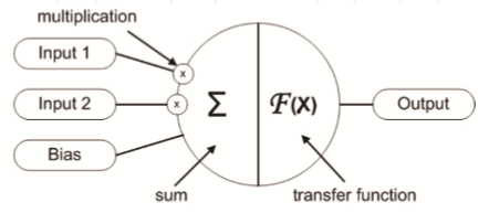
• Dendrite - Inputs : As dendrites passes the information to neurons, the information comes to artificial neurons via inputs which are weighted.
• Soma - Body of Artificial neuron : As Soma processes the information in case of biological neuron, body of artificial neuron summarizes the weighted inputs and apply the transfer function.
• Axon- Output : As Axon takes the information processes by Soma to other neurons, muscles & glands, output, similarly outputs transfer the information to other artificial neurons.

Artificial neuron has three simple sets of rules as shown above - multiplication, summarization and activation. At the entrance of artificial neurons all inputs are weighted, then these weighted inputs and bias are summarized in the central part and at last these sum of weighted inputs and bias is run through the transfer function and output is provided.

Mathematically this artificial neuron can be summarized as :

                                          

The major unknown variable of the model is the transfer functions. This transfer function is chosen on the basis of the problem we are solving. Step function, linear function and signoid functions are generally used in most of the cases. Mostly artificial neurons exploits the non linearity and uses sigmoid functions.

Artificial Neural Networks :

Some of the characteristics of Artificial Neural Networks that mimic the properties of the biological neural network are:

• They exploits the non linearity - They exploit non linearity by interconnection of non linear neurons.
• They have Input-Output Mapping - They have learning capability both "with"(supervised)  a teacher as well as "without" (unsupervised) a teacher.
• They are Adaptive - They can adapt to the changes in the surrounding environment

These interconnected artificial neurons have the capability to solve various real life problems by exploiting the above properties. Below figure shows how these neurons could be interconnected in three different layers - Input, hidden and output layer.


The steps involved to start using the interconnected neurons is to :

• First define the topology or architecture and fine tune that in which way these neurons could be interconnected to form network.
• Teach (train) it to solve the given type of problem

Artificial Neural Networks Topology

There are two basic ways in which artificial neurons could be connected to each other
1) Feed Forward topology
2) Recurrent Neural Network Topology

In the case of Feed forward topology, the information flow from input to output in only single direction(directed acyclic graph)  whereas in case of Recurrent Neural network topology, the information can flow in both the directions (directed cyclic graph). The main advantage of RNN is that they can use their internal memory to process sequence of input. Below figure shows both these topologies.

Feed Forward & Recurrent Neural Network Topology

Different Topology of  Neural Networks :

• Fully Recurrent Artificial Network - This is the most basic topology of recurrent neural network where every basic unit is connected to every other unit in the network.

• Hopfield Artificial Neural Networks - This is the type of RNN where one or more stable target vector is stored. This topology has only one layer with each neuron connected to every other neuron with restriction that no unit has connection to itself & connections are always symmetric. This topology can be used for various pattern recognition problems as it has the memory of target vectors which can be recalled when given similar vector that acts as the cue. 

• Elman & Jordan Artificial Neural Networks: These topology is also referred as Simple Recurrent Network. This is simple three layer artificial neural network that has back loop from either output layer or from hidden layer to input layer through context unit. In case of Elman, back loop is from hidden layer to input layer whereas in case of Jordan back loop is from output layer to input layer. As Elman network is able to store information, it is able to generate temporal and spatial patterns.

• Long Short Term Memory : As the name suggests, in this kind of topology it can remember the value for any length of time and therefore network can process, classify and predict time series with very long time lags. The remembering process is controlled by gates which determine when the input is important to remember, how long the input value to be remembered and when this value to be released to the output.

• Bi Directional Artificial Neural Network : Bi-ANN were invented to increase the amount of input information that can be referred. These consist of two individual interconnected artificial neural networks. These are very useful for the type of prediction where context of the input is important eg - handwriting recognition where knowledge of the current letter can be improved by having details of letter before and after the letter. These are very useful to predict complex time series .

Below is the representation of different topologies of Neural Network :

Fully Recurrent, Hopfield, Elman Recurrent Neural Network Topology

Jordan, Bi Directional & Long Short Term Memory Recurrent Neural Network Topology

Learning :

Once the topology is defined for the Neural network, next step is to train them to solve the given type of problem. One of the important characteristic that artificial neural networks mimic from biological neuron in the brain is their ability to learn. in ANN the learning is mimicked by setting the weights of the connections between the different neurons using algorithms to get the desired output.  

The three major learning paradigms that can be used to train any artificial neural network are as follows :

• Supervised Learning : This is a technique where the desired output is also provided with the input while training the algorithm. The weights of the network is adjusted in such a way to come close to the desired output. Various steps are involved to solve the given problem using supervised learning - Determine the training examples, gather the training data that describe the given problem, describe gathered data set in form understandable to a neural network, do the learning and as the last step validate the output by performing tests.

• Unsupervised Learning : In this technique set of unlabeled inputs are given without setting some relationship between this data. Artificial neural network tries to find some relationship between this data. These are used to solve mostly the estimation problems such as statistical modelling, compression etc. Mostly self organizing maps are used for unsupervised learning algorithms.

• Reinforcement Learning: Reinforcement learning is influenced by the behavioral psychology. It is something how the natural learning works for example kid knows which action to perform again to make others praise/clap for him (reward). In this type of learning the data is not generally given but generated by interaction with the environment. The aim here is to maximize the reward by trying out different options.  Reinforcement learning is mainly suited for problems which include long term versus short term reward trade off. Some of the problems it is applied to are robotics, game theory, telecommunications etc.

Usage of Artificial Neural Networks :

One of the best characteristic of Artificial Neural Networks is their ability to learn form the environment. This is similar to how our central nervous system  or brain works. In artificial neural networks we give input and output to the neural networks and it works on to create the function to generate the optimum output after learning. This is the reason there are good usage of Artificial Neural Networks in the fields which our brain does very good like facial recognition, handwriting recognition, game theory etc.

One thing to note is that selection of particular topology is governed by the type of problem we are solving and the data set available for it. Also complexity of the model that we are choosing to solve the given problem plays the major role. Using very simple model can give poor result and using very complex model to solve simple problem can cause issues during the learning process.

One of the usage of Artificial Neural network is for modelling and representing natural language. Natural language processing has the core usage in many industries like search engine, email categorization, Pharma Co vigilance etc. Wait for my next blog to get the glimpse of usage of Neural Networks for Natural Language Processing.

References :

1. Introduction to the Artificial Neural Networks  By Andrej Krenker, Janez Bešter and Andrej Kos.
2. Wikepedia
3. http://www.theprojectspot.com/

Impose a set of behavioral state-change rules to the random arrays using Python

I was challenged by my mentor to implement the below condition using Python. 

Impose a set of behavioral state-change rules to the random arrays (100 x 100) 

Whenever a square is surrounded by 4 other squares (either adjacent or diagonal) then it retains its value for all future iterations from that point forward. 

All squares that do not become bound in any given iteration, continue changing until they are bound by 4 squares at some future time. 

The goal of this is to initiate a random array, populate it with arbitrary set of numbers from a uniform random distribution [0,1], and to apply the rules below to each square, evaluated on every iteration. 

Below is the pictorial representation of the problem 

While working on the implementation found that this condition is somewhat similar to Conway Game of life. I read some details about the Conway game of life and found it very interesting. Here are  some of the details about the Conway Game of life :

The universe of the Game of Life is an infinite two-dimensional orthogonal grid of square cells, each of which is in one of two possible states, alive or dead, or "populated" or "unpopulated" (the difference may seem minor, except when viewing it as an early model of human/urban behavior simulation or how one views a blank space on a grid). Every cell interacts with its eight neighbours, which are the cells that are horizontally, vertically, or diagonally adjacent.


I tried to implement the behavioral state-change rules using Python. While implementing took help from some of the online posts also. I tried the problem in below two ways by first taking only two states and then in the second attempt tried the rules on the random array. Here are those two approaches :

1) Took only two option of cells to be live or dead and applied the behavioral state change rule.

2) Applied behavioral state-change rules to the random arrays (100 x 100)

Here is the code for both the conditions :

Approach 1: Took only two option of cells to be live or dead and applied the behaviourial state change rule.

################################################################################

# conway-On-Off.py

#

# Author: Ravi Vijay

# 

# Description:

#

# A simple Python/matplotlib implementation of following condition :

#  Whenever a square is surrounded by 4 other squares (either adjacent or diagonal) then it retains its #value for all future iterations from that point forward.  

#  All squares that do not become bound in any given iteration, continue changing until they are #bound by 4 squares at some future time.

################################################################################

import numpy as np

import matplotlib.pyplot as plt 

import matplotlib.animation as animation

N = 100

ON = 255

OFF = 0

vals = [ON, OFF]

# populate grid with random on/off - more off than on

grid = np.random.choice(vals, N*N, p=[0.2, 0.8]).reshape(N, N)

def update(data):

  global grid

  # copy grid since we require 4 neighbors for calculation

  # Putting here the loop to go line by line 

  newGrid = grid.copy()

  for i in range(N):

    for j in range(N):

      # compute 4-neighbor sum (once adjacent & once diagonal) 

      # At boundary condition we wrap around 

      

      # Adjacent Total

      total1 = (grid[i, (j-1)%N] + grid[i, (j+1)%N] + 

               grid[(i-1)%N, j] + grid[(i+1)%N, j])/255

        

      # Diagonal Total  

      total2 = (grid[(i-1)%N, (j-1)%N] + grid[(i-1)%N, (j+1)%N] + 

               grid[(i+1)%N, (j-1)%N] + grid[(i+1)%N, (j+1)%N])/255

      

      

      # Apply rules

      if grid[i, j]  == ON:

        if (total1 !=4) or (total2 != 4):

          newGrid[i, j] = OFF

      else:

        newGrid[i, j] = ON

  # update data

  mat.set_data(newGrid)

  grid = newGrid

  return [mat]

# set up animation

fig, ax = plt.subplots()

mat = ax.matshow(grid)

ani = animation.FuncAnimation(fig, update, interval=200,

                              save_count=200)

plt.show()

Here is the screenshot for the iteration :

Approach 2: Applied behavioral state-change rules to the random arrays (100 x 100)

################################################################################

# conway.py

#

# Author: Ravi Vijay

# 

# Description:

#

# A simple Python/matplotlib implementation of following condition :

#  Whenever a square is surrounded by 4 other squares (either adjacent or diagonal) then it retains its value 

#  for all future iterations from that point forward.  

#  All squares that do not become bound in any given iteration, continue changing until they are bound by 4 squares at some future time.

################################################################################

import numpy as np

import matplotlib.pyplot as plt 

import matplotlib.animation as animation

N = 100

m=100 # Matrix Size

c=5   # Number of Colors

# populate grid with random on/off - more off than on

grid = np.random.randint(c, size=(m, m))

def update(data):

    global grid

  # copy grid since we require 8 neighbors for calculation

  # and we go line by line 

    newGrid = grid.copy()

    for i in range(m):

      for j in range(m):

      # apply rules

          if ((grid[i, (j-1)%N] == grid[i, (j+1)%N] == grid[(i-1)%N, j] == grid[(i+1)%N, j]) 

              or (grid[(i-1)%N, (j-1)%N] == grid[(i-1)%N, (j+1)%N] == grid[(i+1)%N, (j-1)%N] == grid[(i+1)%N, (j+1)%N])):

                newGrid[i, j] = grid[i,j]

                

          else:

            newGrid[i, j] = np.random.randint(c, size=(1, 1))

            

  # update data

    mat.set_data(newGrid)

    grid = newGrid

    return [mat]            

  

# set up animation

fig, ax = plt.subplots()

mat = ax.matshow(grid)

ani = animation.FuncAnimation(fig, update, interval=50,

                              save_count=50)

plt.show()

Below is the screenshot of few of the iterations :

Paper Review - Machine Learning : a review of classification and combining techniques

Got the chance to go through this paper on Machine Learning.  It was recommended to me by my mentor. This is a very good paper to understand the whole perspective on Machine learning. Author has summarized very well about the supervised learning methods and when you should consider using each method.

It took me some time to go through the whole paper and also I need to come back on various topics in the article to have the better understanding. I highly recommend this paper to all those who are starting with the machine learning journey and would like to see the importance of each ML algorithm for supervised learning. 

These are some of the points that I would like to summarize :

Supervises Learning : If the instances are given with known labels

Unsupervised Learning : Instances are unlabeled.

The main aim to go through various ML algorithms is to understand the strengths and limitations of each algorithms. While solving the problem we should consider using the combination of algorithms for better accuracy.

Just using one algorithm and trying to increase the accuracy may not help always.

Issues with supervised learning :

The first step towards using ML is to collect the dataset.
While preparing the dataset try to find out the fields which are most informative. If that information is not available we can use brute force method ie measure everything in the hope that the right feature can be isolated.There are challenges with the brute force as it requires pre processing.

Some of the methods used for pre processing & cleansing of dataset described by author are :

• Variable-by-variable data cleansing
• Use of visualization tool.
• Instance selection to  handle noise - This is more of the optimization problem. For sampling the instances methods can be used such as Random sampling, Stratified sampling etc
• Handling the incomplete feature values - Methods like ignoring features with unknown values, Selecting most common feature value, mean substitution, regression & classification, treating mission values as special values can be used.
• Feature subset selection
• Feature construction/transformaton

Algorithm Selection :
The author talks about the importance of using the right algorithm. The prediction accuracy is the main criteria for the classifier evaluation. The techniques generally used for the classifier accuracy are - split the training set, cross validation method, Leave one out method. Leave one out is the special case of cross validation process. The disadvantage of this method is that it requires lot of computation but gives the most accurate estimate of the classifiers error rate.

Supervised Machine Learning techniques -

1) Logic Based Algorithms - Symbolic learning Method

a) Decision Trees:  These are the trees that classify instances based on the feature values. The decision trees are easy to comprehend.

b) Rule based classifier: Here the author talks about the difference between the Decision tree and the Rule based classifiers. The main difference emphasized by author is that the decision tree evaluate the average quality of number of disjoint sets whereas the rule classifier only evaluate the quality of the set of instances that is covered by the candidate rule. 

Another difference is that the decision tree uses the Divide & conquer approach while the Rule based classifier uses the Separate and conquer method. For smaller datasets its always advantageous to use the divide and conquer method.


c) Inductive Logic Programming : Some of the characteristics emphasized by author for Inductive Logic Programming are - Expressive representation, Ability to make use of logically encoded background knowledge & extensive use of Inductive Logic programming in Relational Data Mining.


2) Perceptron Based Techniques :

Perceptron is described as  - If X1 to Xn are input features and W1 to Wn are prediction weights/vectors, than perceptron algorithm computes the sum of weighted inputs iXiWi and adjust the threshold : if sum is above threshold output is 1 else 0.
Author describes the advantage of  perceptron based technique when the number of features are high.
Some of the disadvantages are that it cannot deal with numerical problems and also perceptron like methods are binary.

Neural Networks :

If a straight line can be drawn to separate the input instances into correct category, perceptron culd find the solution. IF the straight line cannot be drawn, it is difficult to reach the point where all instances are classified properly.
Artifical Neural Networks helps to solve this problem.

Neural network consist of 3 types of units - Input Unit, Output Units and in between of input & output units, hidden units are present.

ANN depends on 3 fundamental aspects - Input & activation function of the unit, network architecture and weight of each input connection.

The most common method used to find the value of the weight is Back Propogation Algorithm.

The major disadvantage of the ANN is their lack of ability to reason about their output in a way that can be effectively communicated.



3) Statistical Learning Algorithms :
The author describes that as compared to ANN, statistical approach define the probability model to define if a an instance belong to a particular class. Bayesian networks & Instance based method belongs to this category.

Bayesian Network :

Bayesian Network is a probabilistic graphical model that represents a set of random variables and their conditional dependencies via a directed acyclic graph (DAG). For example, a Bayesian network could represent the probabilistic relationships between diseases and symptoms. Given symptoms, the network can be used to compute the probabilities of the presence of various diseases.

Author explains that computational difficulty in exploring a previously unknown network is one of the limitation of Bayesian Network.

Author also emphasizes on the feature of BN as compared to decision tree or neural networks - possibility of taking into account prior information about a given problem.

It is also important to note that BN are not useful for data sets with many features.


Naive Bayes Classifier :

NB classifiers belongs to the family of Bayesian Network with strong independence assumptions between the features. They are composed of DAG's with single parent and many children with the assumption of independence among the child nodes.

Author also emphasizes that the assumption of independence among child nodes is always wrong and that is the reason that NB classifiers are less accurate as compared to other sophisticated algorithms like ANN.

Some of the methods used to overcome the independence assumption and improve the classifier accuracy in research are - CR method (Network has the limitation that each feature could be related to only one other feature), Selective Bayesian Classifier ( to include a feature selection stage. This is to improve the classification performance by removing the irrelevant features).

Author emphasizes that the majr advantage of NB classifier is the short computational time for training.

Instance-based learning : 

These are also called the lazy learning algorithms as they delay the generalization process till the classification process. They require less computational time during the training phase and more during the classification phase due to this reason.
One of the example talked about the author is k nearest neighbor. Some of the characterstics of K nearest neighbor are - they have lasrge storage requirement, sensitive to choice of similarty fnction, lack well defined method to choose k ie its nearest neighbors.


4). Support Vector Machine 

SVM runs around the concept of margin. Author describes that if we consider the hyperplane and the margin that separates two data classes, maximizing the margin can help in to reduce the upper bound on expected generalization error.
SVM is very useful where the number of features are large as compared to number of training instances. The author describes how Sequention Minimal Optimization can relatively quickly solve the SVM QP problem.


5). Characteristics of each Algorithm

Author described the characteristic of each algorithm and have put the point of view on where & why to use each algorithm. I have summarized the highlight of that below :

SVM & Neural Networks  - Multi-dimensions & continuous features.
Logic Based - Discrete/categorical features
SVM - Requires large sample size

KNN - very sensitive to irrelevant features, lot of storage space, require complete set with missing values eliminated.
Neural Networks - presence of irrelevant features can make training inefficient, require complete set with missing values eliminated.

Naive Bayes - High Bias, little storage, robust to missing values.
Decision Tree, Neural Network, SVM - High Variance



At the end,  author summarizes how these machine learning algorithms could be combined together to get the better outcome.


Thoroughly enjoyed reading and summarizing the article here in this blog !

Plotting Heat Map in Python

Python is the scripting language generally used by Data Scientists for the Analytics purpose. As I was making my journey to get expertise in Machine Learning & Analytics, started trying my programming skills using Python.
I used the following resources to get me started -

1) Pycharm - https://www.jetbrains.com/pycharm/
It provides the complete IDE for python and easy to use. There are some short exercises in this which can help in making the quick start on Python programming.

2) Coursera Course on Python (Coursera.org)
Few courses on Coursera are available that helps you take deep dive in Python.


As the first challenge to test my Python skills, tried to achieve following task :

(i) Create a 2-dimensional array of size 100x100 and populate it with random floating points between 0 and 1 (inclusive (i.e., [0,1]); 
(ii) plot the 2d array using any python library, to create a visual “heat map” representation of the data; 
(iii) write a loop that refreshes the numbers in the array and replots the heatmap each time the array is repopulated.  


I tried this program in ipython notebook.




%matplotlib inline
import matplotlib.pyplot as plt
import numpy as np
for i in range(1,5):
    data = np.random.rand(100,100)
    fig, ax = plt.subplots()
    ax.set_title("Heat Map Assignment:")
    heatmap = ax.pcolor(data)







Some of the points to note :
%matplotlib inline
Helped me to plot the heatmap inline in the ipython notebook only instead of opening the new browser window each time.

matplotlib library :
It provides the various functions to plot the graphs.

numpy :
Used the numpy here as it provided the easy way to create the multi dimensional array and populate it with random numbers. Only thing that I missed here is that how to make upper limit inclusive while populating the array with random floating point numbers. Still trying to find a way ...




This is the output :